Hello World! 🌎

Hello internet, welcome to my personal website 🐣! First time doing this, let’s see how it goes!

Display some Math: #

Einstein’s famous Mass-energy equivalence formula 🌌:

$$ E = mc^2 $$

From wiki: The formula defines the energy E of a particle in its rest frame as the product of mass m with the speed of light squared (c²).

The 🔔 Curve: With the probability density function:

$$ f(x | μ, σ^2) = \frac{1}{\sqrt{2 \pi \sigma^2}} \exp \left( -\frac{(x - μ)^2}{2 \sigma^2} \right) $$

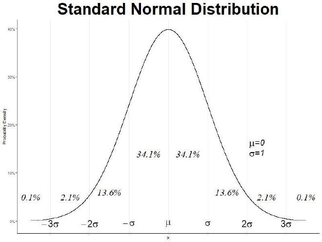
Where μ is the mean or expectation of the distribution and σ is the standard deviation. i.e. variance of σ². It is also known as the Gaussian Distribution or more commonly known as the Normal Distribution. An example graph of the function:

Embedding code block #

This is the R code used to generate the above graph.

#Clear console and environment
rm(list = ls())
cat("\014")
#attach required library
library(ggplot2)
library(dplyr)
#set mu and sigma parameters for the Normal Curve
mu<-0
sigma<-1
#generate data
x<-seq(-4*sigma,4*sigma,0.0001)-0.5
y<-dnorm(x,mu,sigma) #density function
data<-cbind(x=x,y=y) %>% data.frame()
xlab<-c(expression(-3*sigma)
 ,expression(-2*sigma)
 ,expression(-sigma)
 ,expression(mu)
 ,expression(sigma)
 ,expression(2*sigma)
 ,expression(3*sigma)
)
p_lab<-pnorm(seq(-3*sigma,3*sigma,sigma),mu,sigma)
#Plot:
ggplot(data,aes(x,y))+
#Plot area settings:
 theme_classic()+
 theme(plot.title=element_text(size=40,face="bold",hjust=0.5)
 ,panel.grid.major.x=element_line(size = (0.2))
 ,axis.text.x=element_blank())+
 ggtitle("Standard Normal Distribution")+
 xlab("x")+
#text for the sigma labels
 annotate("text",
 x = seq(-3*sigma,3*sigma,sigma),
 y = rep(-0.005,7),
 label = xlab,
 family = "", fontface = 3, size=8) +
#text for the density values at each n*sigma area
 annotate("text",
 x = c(seq(-3*sigma,3*sigma,sigma)-0.5*sigma,0.5*sigma+3*sigma),
 y = round(c(p_lab[1],diff(p_lab),p_lab[1]),1)^2+0.05,
 label = paste0(round(c(p_lab[1],diff(p_lab),p_lab[1])*100,1),"%"),
 family = "", fontface = 8, size=8) +
#display parameter values
 annotate("text",
 x = rep(2.2*sigma,2),
 y = c(0.16,0.14),
 label = c(expression(paste(mu,"=")),
 expression(paste(sigma,"="))),
 family = "", fontface = 3, size=8) + 
 annotate("text",
 x = rep(2.4*sigma,2),
 y = c(0.164,0.143),
 label = c(mu,sigma),
 family = "", fontface = 3, size=7) + scale_x_continuous(breaks=seq(-3*sigma,3*sigma,sigma),limits=c(-3.5*sigma,3.5*sigma))+
 ylab("Probability Density")+
 scale_y_continuous(labels=scales::percent_format(accuracy=1))+
 geom_line()

Some Linear Algebra: #

To find a plane of best-fit.

Given a data vector with n samples and p parameters:

$$ \begin{Bmatrix} y_i, x_{i1},\cdot \cdot \cdot ,x_{ip} \end{Bmatrix}^{n}_{i=1} $$

Where the dependent variable y and the p-size vector of regressors x are assumed to be a linear relationship. Where the error variable ε was modeled such that it is the minimum and ideally it experiences an unobserved random variable. i.e. “noise”.

Then ideally we want to find β where the model has the form:

$$ y_i = \beta_0 + \beta_1 x_1 + \cdot \cdot \cdot + \beta_p x_{ip} + \varepsilon_i = x^T \beta + \varepsilon $$

Or simply

$$ y = X \beta + \varepsilon $$

Where

$$ y = \begin{Bmatrix} y_1, \cdot \cdot \cdot y_n \end{Bmatrix}^T $$

$$ X = \begin{pmatrix} x^T_1 \\\ \cdot \\\ \cdot \\\ \cdot \\\ x^T_n \end{pmatrix} = \begin{pmatrix} 1 & x_{11} & \cdot\cdot\cdot & x_{1p} \\\ & & \cdot & \\\ & & \cdot & \\\ & & \cdot & \\\ 1 & x_{n1} & \cdot\cdot\cdot & x_{np} \end{pmatrix} $$

and

$$ \beta = \begin{pmatrix} \beta_0 \\\ \beta_1 \\\ \cdot \\\ \cdot \\\ \cdot \\\ \beta_p \end{pmatrix} , \varepsilon = \begin{pmatrix} \varepsilon_1 \\\ \cdot \\\ \cdot \\\ \varepsilon_n \end{pmatrix} $$

Hence for a line, you are solving for the equation with one parameter $$y = \beta_0 + \beta_1 x$$ and for a plane there will be two parameters. $$y = \beta_0 + \beta_1 x_1 + \beta_2 x_2$$

Least-squares estimation: #

Since y and x are assumed to be a linear relationship and we would like to find the “best” β which solve the system of equations and to minimize ε. Hence let: $$ \varepsilon = L(X,y,\hat{\beta})=\left | X\hat{\beta}-y \right |^2 = (X\hat{\beta} - y)^T(X\hat{\beta}-y) \ $$ $$ = y^Ty - y^TX\hat{\beta} - \hat{\beta}^TX^Ty + \hat{\beta}^TX^TX\hat{\beta} $$ Where L is called the Loss function, essentially the error term is modeled with the input X, y, β. Since X, y is the original data we want to “fit”, therefore we can find the “best” β at which L(X, y, β) is minimized.

Hence the first derivative of L(X, y, β):

$$ \frac{\partial L(X,y,\hat{\beta})}{\partial \hat{\beta}} = -2X^Ty+2X^TX\hat{\beta} $$

Since X, y is fixed and known and we only interested in the “best” β therefore:

$$ \hat{\beta} = (X^TX)^{-1}X^Ty $$

This is the case for the Simple Linear Regression.

This concludes the Hello World! 🌎 Thank you for reading!